Home and Learn: Power BI 2023
Power BI 2023 KPI Visuals
Let's see how to add a KPI to a Power BI dashboard. First, though, what is a KPI?
A KPI is a way to see if a target has been met or not met. (The letters stand for Key Performance Indicator.) Take the image below as an example:

In the B column are the names of salespeople. The C column lists what their sales figures were. The D column lists what the individual sales targets were. With a KPI visual, we can click on the name of a salesperson and see at a glance if they have met their target. In the image below, we've selected the salesperson Blythe Smethurst. We can quickly see that he has met his goal of 2871 sales:

The Guage below the KPI is another visual we can add to display target information. You'll see how to add one of those, too.
In the next image, we've selected the salesperson Esme Yukhin. You can see that this salesperson has not met the target sales of 3302, and has fallen way short.

Let's see how to add a KPI to a dashboard.
Here's the data you need for this tutorial (right-click, Save As):
As in other lessons, load the Text/CSV file into Power BI. There's no need to transform the data, so just load it. Once it's loaded, the Data panel on the right of Power BI should look like this:

Let's add a table first, so we can see the data and select sales staff from it.
You've added tables before in previous sections, so we won't go fully into it. But, from the Home ribbon, add a Table visual to your dashboard:
For the Columns, add the following data: Salesperson, ActualSales, TargetSales. Your table should look like this, when you're done:


When you click on the KPI item, you should see a blank KPI visual appear on your dashboard:

The three sections you can add data to are Value, Trend Axis, and Target. For the Value item, this is for your Actual Sales; for the Target item, you want your Target Sales here; for the Trend Axis, this where you would put a date field, if you had one. So you want to measure a Value over a certain period (Trend) and display a Target.
Click the Add data button under Value and select the ActualSales column from your table. For the Trend Axis, click the Add data button and select the ID column from your table. For the Target section, click the Add data button and add the TargetSales column. Your KPI will then look like this: (If it doesn't, click Blythe from the salespeople.)

Remember: as we did in a previous lesson, you can rename the items in the data flyout. Right-click where it says Sum of Actual and Sum of Target. From the menu that appears, select Rename for this visual. Type a new name for the item. In the image below, we've renamed to Actual Sales and Target Sales:

(You can rename table column headers using the same technique: toggle the data flyout on the table, right-click, rename for this visual.)
From your table, select the second salesperson. The KPI will update to this:

The big red numbers are showing Bryna's sales figures of 1969. However, the sales target (goal) was 2941, which is 33.05 percent short of the target. Because the KPI was missed, the large number is in red. But you can change these colors, and tweak the KPI card to your liking.
Format Power BI 2023 KPI cards
Click the paintbrush icon to toggle the Format flyout. You should see this:

There are four out of five options already selected. Uncheck the Icons item and you should see the red exclamation mark disappear. (The icon is an exclamation mark, if the target is missed, a green tick if hit.) Uncheck and check the other to see what they do.
But click the More options button. The format pane should open on the right of Power BI:

Expand the Icons item:
![]()
Sadly, you can't select a different icon. You can only change its size.
Expand the Title section at the top and you can change the title of your KPI to anything you like. In the Image below, we've changed ours to KPI Targets:

Now expand the Trend axis item:

This section is where you can change the colors for your Power BI KPI card. The default is to have high as good. If a target has been met, the text color will then be green. If the target has not been met ,then the color will be red. You can change these colors to anything you like by selecting a new color from the dropdown lists.
Sometimes, however, you want low as good. For example, you're a police chief putting together a dashboard and wish to measure the number of complaints your officers have received. In this case, high is very definitely not good. If an officer has received a high number of complaints, you don't want to see a green tick in their KPI. That would create quite the wrong impression! To change it from High is Good, click the dropdown. There is only one other option - Low is Good.
KPI Target Label
The target label is the text below the headline number. You can change and format this text to anything you like. Expand the Trend label item:
The default text is Goal. In the image below, we've changed it to Target. We've also changed the default font size from 12 to 14, and picked a different color.

Here's what our KPI card looks like:

(You can add a visual border to any Power Bi visual by expanding the Size and style section, then Visual Border. We did size and style formatting in a previous lesson, so won't go over it again.)
And that's pretty much it for KPI cards. There's not much you can do with the formatting, but they do come in handy, if you need to measure and display targets.
Power BI 2023 Dashboard Gauge
Let's add the gauge, just so we can have another visual that measures targets.
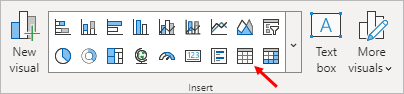
Click on a white area of your dashboard to deselect the KPI. From the
Home ribbon at the top of Power BI, click the Gauge item
on the Insert panel:

The default gauge will look like this:

The Value for the gauge is the Actual Sales; the Target value is the figure you are trying to hit (Target Sales, for us). You can add a minimum value and a maximum value. We'll do this through the formatting panel.
Click the Add data button under Value. Select the ActualSales column from your data table. Your gauge will then look like this:

Now click the Add data button under the Target value heading. Add the TargetSales column from your data table. The gauge will then turn into this:

Click the Blythe Smethurst item in your table visual. The gauge will update to this:

The gauge is showing Blythe's sales figures in the bottom center of the gauge, with his target figure on the gauge itself. The line on the gauge is the target figure. You can quickly see that this salesperson has exceed the target figure, and by how much. The minimum value of 0 and the maximum value of 6200 are not what we'd like, however. Let's change them.
Click the paintbrush icon to toggle the formatting flyout. It should look like this:

There four items preselected for you: Title, Data labels, Target label, and Callout value. Check and uncheck these items to see what the four items do.
But click the More options button to activate the Format panel on the right of Power BI:

The Title options are the same ones as before. Expand the Gauge axis item:

The Gauge axis section is where you can set a minimum and maximum value for your gauge. The default is auto. Change these to reflect the minimum and maximum values from the table. In the image below, we've set minimum to 1500 and maximum to 3400:

The gauge visual on your dashboard will update to this:

Now the numbers at the bottom of the gauge are better for our table visual.
Now expand the Colors section:

You can change the colors of your gauge here, both the fill color and the target color (the line). In the image below, we've gone for a purple theme for our gauge:

Explore the other sections for yourself: Data labels, Target label, and Callout value. The options for these sections should be familiar to you now.
Replacing the Power BI KPI Icon
Although you can't select a different icon for the KPI card (the green tick and the red exclamation mark), you can switch it off and replace it with a suitable image. It's a bit of a hack, though, and we'll need to add a new column to our data table, and write some DAX. But let's give it a try.
What we want to do is to have an emoji at the bottom of the KPI card. This, when the target has been met:
![]()
And this when it hasn't been met:
![]()
First, select your KPI card. Click the paintbrush icon to toggle the Format flyout. Deselect the Icons item:
![]()
Add a New Column and Create the DAX Measure
Now we need to create a DAX measure. For the measure, we want to say this: If the Actual Sales figure is greater than or equal to the Target Sales figure, then display a positive emoji. If it's not, display a negative emoji. The DAX code would be this:
IF( KPI_DATA[ActualSales] >= KPI_DATA[TargetSales], "POSITIVE", "NEGATIVE" )
If you've ever done any Excel IF statements, then this code should be familiar to you. The syntax is:
IF( YOUR_CONDITION_HERE, WHAT_TO_DO_IF_TRUE, WHAT_TO_DO_IF_FALSE)
However, we can't just create a new measure by itself for this. We need to add a column to our data table and then write a measure for that new column.
Let's add the new column.
In the Data panel on the right of Power BI, right click your table name. From the menu that appears, select New column:

When you click on New column, you should see a formula bar at the top of Power BI. Enter the following, stopping when you get to the double quote at the end:
Smiley = IF(KPI_DATA[ActualSales] >= KPI_DATA[TargetSales],
"
![]()
After the double quote, press the WINDOWS key on your keyboard. Keep the WINDOWS key held down and press the full stop/period key on your keyboard. You should see a popup appear with lots of emojis on it:
![]()
You can select an emoji on the smiley face tab, or select a different tab at the bottom to see more emojis.
Select the emoji you want. It's a little bit fiddly to add the emoji to the formula because you can't just double-click when you've selected an emoji. Nor can you just hit the Enter key on your keyboard. This won't add the emoji to your formula. Instead, select an emoji and then click back inside the formula bar.
Now type a double quote and then another comma:
![]()
That's the first emoji, the one if ActualSales are greater than or equal to TargetSales. After the comma on the end, type another double quote. Now add your second emoji, the one you want if the target is not hit. After the second emoji, you need another double quote and then a round bracket to close the whole thing off. Hopefully, you'll end up with something like this, depending on your selected emojis:
![]()
After all that, click the tick on the left of the formula bar, or just press the Enter key on your keyboard.
To see your new column, click the Data view icon on the left of Power BI:
![]()
As you can see, we have a new column called Smiley, which was the name of our measure. In this column is an emoji, a different one, depending on if a target was met.
Now let's put this column to work.
Click back into Report View, so that you can see your dashboard. Add a Card visual to your dashboard. From the flyout, click the Add data button. From the Data flyout, select your new Smiley column:
![]()
When you select the Smiley column, your card will update. Here it is with Blythe Smethurst selected in the table visual:
![]()
Click the paintbrush icon to see the Format flyout. From the Format flyout, uncheck the Category label item. The text First Smiley will disappear:
![]()
Now make your card smaller by adjust the round white circles, which are sizing handles. (Hold your left mouse button down on a sizing handle. Drag to resize.)
The size of the Smiley itself may need adjusting. To do that, click the More options button to display the Format panel on the right of Power BI. Expand the Callout value section and type a new font size. In the image below, we've went with a font size of 20:
![]()
Once your Smiley is nice and small, drag and drop it onto the KPI visual:
![]()
Now select different salespeople from your table visual. You should find that the smiley updates, depending on if that salesperson hit or missed their target.
And that's it for KPI visuals in Power BI 2023. Play around with them and see what you can come up with.
<--Back to the Power BI Contents Page