Home and Learn: Power BI 2023
Power BI 2023 Table Formatting
In a previous lesson, you added a table visual to a Power BI dashboard. In this lesson, you'll learn how to format your tables.
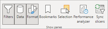
First, create a table, just like you did earlier. With the table selected, bring up the Format panel. To do that, click the View menu at the top of Power BI. Toggle the Format option on the Show Panes panel:
Now Study this table:
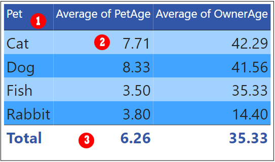
The numbers in the image refer to the following sections of the Format Panel.
- Columns Headers
- Values
- Totals
Let's go through them.
1) Table Column Headers in Power BI
In the image above, the background color for the column headers is a dark blue. The font color is white. To change your table header, from the Format panel on the right, expand the Column Headers section:
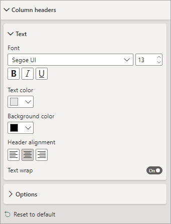
You can select a font and a font size. Change the Text color and the Background color to anything you like.
2) Table Cell Values in Power BI
The Values going into each cell of each column can be changed by expanding
the Values > Values section of the Format panel:
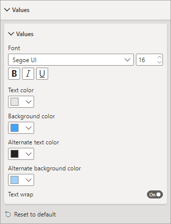
As well as the font and font size, you can change the text and background colors for alternate rows of your table.
3) The Totals Row in a Power BI Table
The bottom row of the table is usually reserved for a Totals row. You can format this by expanding the Totals > Values section of the Format panel:
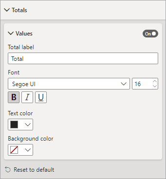
If you don't want a totals row, simply toggle the Values button to OFF.
The Total Label is the text in the first cell of the bottom row. If you want to change the text from the default Total to something else, simply type your new text into the Total Label text box.
Again, you can change the font and font size of the row. You can also select a text color and a background color.
Now let's look at some more table formatting options.
Style Presets for a Power BI Table
If you don't want to go to the trouble of formatting the table yourself, there are some presets you can choose from. Expand the Style Presets section and then click the dropdown to see a list of styles:

The default is None. But you can choose from Minimal, Bold Header, Alternating Rows, Contrast Alternating Rows, Flashy Rows, Cold Header Flashy Rows, Sparse, and Condensed.
Try the out and see what they look like.
Power BI Table Title
If you want, you can have a title at the top of your chart. To do so, expand the Title section of the Format panel:
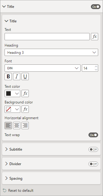
You need to toggle the button to ON, as the title is off by default. But you can have a title, and a subtitle. You can add a divider under the title, and adjust the spacing.
Specific Column Section of the Power BI Table Formatting Options
You can format individual columns in your table. Expand the Specific
Column section in the Format panel:
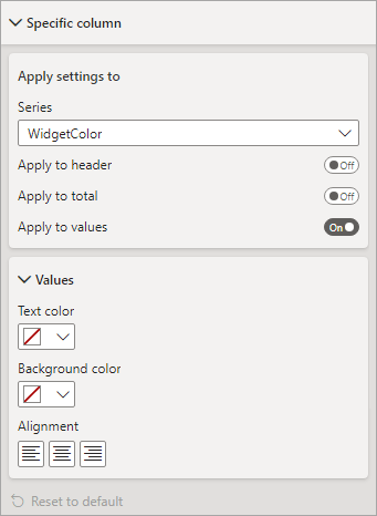
Click the dropdown at the top, under Series. You'll see a list of all the columns in your table. There's a Values section below the Apply Setting To section. The Values section is where you select a Text and Background color, as well as set the alignment. If you want to apply these formatting options to the table header, toggle the Apply to header button to ON; if you want to apply these formatting options to the Totals row at the bottom of the table, toggle the Apply to total button to ON.
Cell Elements Section of the Power BI Table Formatting Options
You can set some extra formatting for the individual columns in your table. Expand the Cell Elements section:
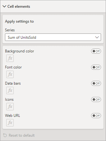
Click the dropdown under the Series heading to see a list of all your columns.
(If your cells have numbers in them, you'll get an extra item - Data bars.)
Toggle the buttons to ON to enable to induvial items.
Here's a table where the column contains numbers, and the Data Bars item toggled to ON.
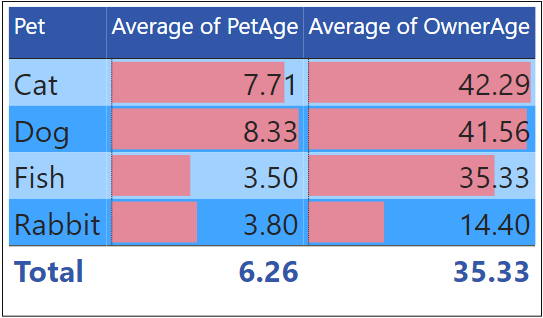
To change the colors of the bars. Click the FX button. You'll see this dialog box:
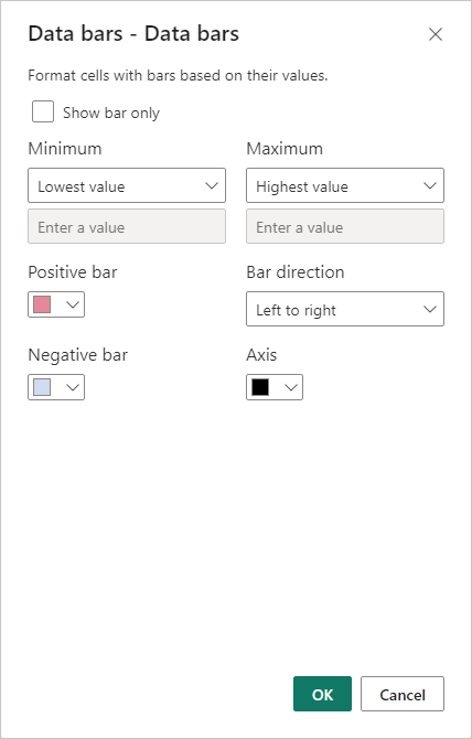
If you don't want numbers at all, check the box at the top Show bars only. You can change the color of your bars. You can have different colors for positive values and negative values. If you only want bars if a value falls between certain numbers, set the numbers in the Minimum and Maximum boxes. The bar direction can be either Left to right or Right to left.
Power BI Table Cell Icons
The Icons item is an interesting one on the Cell Elements section. Toggle the button to ON to see what the default icons look like:
![]()
Click the FX button to see the following dialog box appear:
![]()
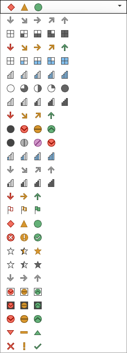
Click the Style dropdown to see a list of available icons:
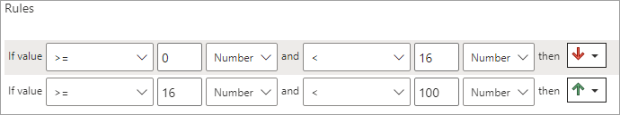
The Rules section at the bottom is where you can specify values based on a condition. For example, you might want a particular icon to appear only if the value in the cell is, say, between 0 and 16. You might want a different icon if the value is greater than this. In the image below, we've added a green up arrow if the value is greater than 16 and red down arrow if the value is less than 16:
And here is the resulting table:
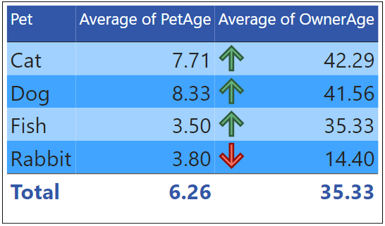
You can really bring a boring Power BI table to life with a bit of formatting!
In the next lesson, you'll see how to work with more than one table for your Power Bi dashboards.
<--Back to the Power BI Contents Page