Home and Learn: Microsoft Excel Course
Excel Confidence Intervals
We've covered Standard Deviation and Standard Error in previous lessons and have a spreadsheet with student scores. Now we're going to explore something called confidence intervals. We'll use our student scores spreadsheet in this lesson. If you haven't yet completed this, the link is here:
Confidence Intervals are a measure of how confident you are that your data is a good representation of the population mean. It's expressed as a percentage. You can then say that you're 95% certain, or 97% certain, or 99% certain, that the true mean is between, say, 45 and 55. So, confidence expressed as a percentage and two numbers used for intervals.
In other words, you're trying to guess the true mean when you don't know what it is. Confidence Intervals are a measure of how accurate your guess is. The narrower the two values (between 45 and 55, for example) the more accurate you are in relation to the true mean. Think about our example of trying to get the Mean height of everyone on the planet called Dave. An impossible task. But you can survey a sample of people called Dave. The more Daves you survey the narrower your confidence intervals will get.
Let's see how to calculate confidence intervals in Excel. We'll work out a confidence interval for all those students whose names begin with the letter A.
In cell G4 of your spreadsheet, enter the text Confidence Interval (A's).
The first formula we're going to use is this:
CONFIDENCE.T(alpha, standard_dev, size)
The gets you something called a T-distribution. The alternative is a z-distribution, which is CONDIDENCE.NORM in Excel. We're using the T version because we have a fairly small sample size of ten students. So, use CONFIDENCE.T when your sample is less than 30. For larger sample sizes, use CONFIDENCE.NORM. You'll see how to use this later.
In between the round brackets of CONFIDENCE.T you need three things:
- A probability value, called the alpha
- The standard deviation of your sample
- How many values are in your sample
The alpha is also known as a p-value. This is the percentage you want, expressed as a decimal. We're going with 95%, which is the most common figure use. Therefore, the figure we'll use here is 0.05. If you want to be confident to 99%, you'd use 0.01.
For the standard deviation, we'll use Excel's STDEV.S, which is used for a sample of the whole population. (Our whole population is 50 students.)
We can get the size value like last time, by using the Excel COUNT function.
So, in cell G5 of your Student Scores spreadsheet from the previous lessons, enter the following formula:
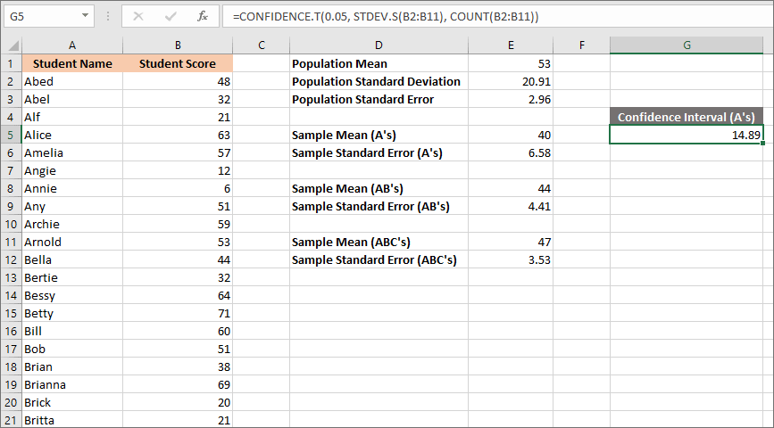
=CONFIDENCE.T(0.05, STDEV.S(B2:B11), COUNT(B2:B11))
Press the enter key on your keyboard and you'll get a figure of 14.88675883. Your spreadsheet should look like this one below (we've reduced the number to 2 decimal places):
So, what do we do with this confidence interval of 14 point something? Well, we're trying to get two numbers: a lower figure for the population Mean and a higher figure. The next step, then, is to deduct 14.89 from the sample Mean of the A's, which is 40. Then we can add 14.89 to 40 to get the higher number.
In cell H4, enter the text Lowest. In cell H5, enter this formula:
= E5 - G5
You should get a really long number, 24 point something. (Widen the H column, if you see a lot of # symbols instead of a number.) You can reduce this to no decimal places via the Number panel of the Home ribbon:
Keep clicking the right arrow until the number in cell H5 says 25. Your spreadsheet should look like this:

Now enter the text Highest in cell I4. To get the highest figure, enter this formula in cell I5:
=E5 + G5
Press enter and then reduce the number of decimal places again. You should get a figure of 55 and your spreadsheet will look like this:
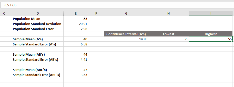
So, we have a low figure of 25 and a high figure of 55 for our confidence intervals. This means we think our population Mean (the one with 50 students) will fall between these two numbers. In fact, we're 95% certain that it will. (To be more accurate, we say that if we took 100 such samples then 95 of them would agree that our population Mean is in the range 25 to 55.)
However, that range, 25 to 55, is a bit on the large size, at 30 points. Is there any way we can reduce it?
To get a narrower range, we need to include more data. Let's see what happens when we include students whose names begin with the letters A and B.
In cell G7, enter Confidence Interval (B's). In cell G8, enter this formula:
=CONFIDENCE.T(0.05, STDEV.S(B2:B21), COUNT(B2:B21))
Same as before, but this time we're covering the range of cells from B2 to B21, where all our A and B students are.
Press enter and you'll get a figure of 9.23 when reduced to 2 decimal places. Your spreadsheet will then look like this:

We can get the low and high figures like we did before.
In cell H7, enter the text Lowest. In cell H8, enter this:
=E8 - G8
In cell I7, enter the text Highest. In cell I8, enter this:
= E8 + G8
The new figures will be 34 to 53, when you reduce them to no decimal places. Your spreadsheet will look like this:
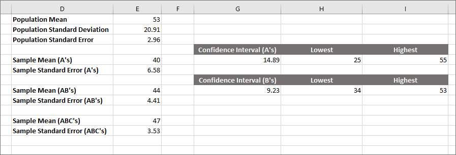
So the estimate of the true population Mean is now between 34 and 53, using a 95% confidence rating. (Remember: this means if you had 100 similar samples, 95 of them would agree.) This is an improvement on our old figure, when we used only 10 students. We're getting narrower. But can we go any lower?
What we'll do now is to use 30 values, those students whose names begin with A, B, or C. This time, because we have 30 students, we'll use the Excel's other CONFIDENCE function, CONFIDENCE.NORM. The rest is pretty much the same.
Enter the following text headings in cells G10 to I10: Confidence Interval (ABC's), Lowest, Highest.
In cell G11, enter the following formula:
=CONFIDENCE.NORM(0.05, STDEV.S(B2:B31), COUNT(B2:B31))
Press enter to get a figure of 6.91 when reduced to 2 decimal places. Your spreadsheet will then look like this one:

The Mean for this sample is 47, which is in cell E11. For the lowest figure, enter this in cell H11:
=E11 - G11
For the highest figure, enter this in cell I11:
=E11 + G11
Press enter and reduce to no decimal places. When you do, here's what your spreadsheet should look like

We now have a low of 40 and a high of 54. These figures are much narrower than the ones we started out with. Bear in mind what we're doing here: trying to estimate what the true population Mean is with a degree of certainty, 95 certainty, to be exact. We can see our true population Mean at the top. It was 53. So the estimate is pretty accurate now. Often, though, you won't know the true population Mean. Think back to our hypothetical population of people called Dave. We wanted to estimate the Mean height of everyone on the planet called Dave. This shows you that you don't have to conduct that impossible task. All you need to do is to take a large enough sample. The larger the sample you take, the narrower you're estimate will be of the Mean. (It needs to be a representative sample, however. It's no good just asking basketball players who are called Dave what their height are - your sample will be badly skewed.)
One more warning to bear in mind with what we've just done. You should only apply these confidence intervals to data that has normal distribution, or something that resembles a normal distribution. (Did you get an OK Bell Curve using the techniques outlined in a previous lesson?)
In the next lesson below, you'll learn about something called Binomial Distribution. This is used to calculate the chances of something happening. What are the odds of that?!
<--Back to the Excel Contents Page