Home and Learn: Microsoft Excel Course
Excel Quartile, Excel Interquartile Range
In this lesson, you'll use Excel to work out the quartiles of a series of numbers. You'll also learn how to calculate the Interquartile Range. What fun!
What is a Quartile?
As its name suggest, a quartile is a way to divide a series of numbers into quarters. And you want each quarter to have the same number of values. So you wouldn't have, say, 4 numbers in the first quarter and 5 in the second quarter.
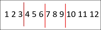
Quartile
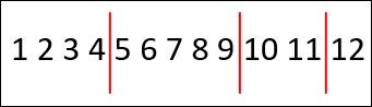
Not a Quartile
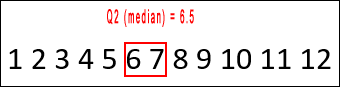
Notice that a quartile only has three points (dividing lines). These are usually labelled Q1, Q2, and Q3. Q2 is the middle number (the median) or numbers. In the image below, you see an even number of values. In this case, to get Q2, you take the middle two numbers and divide by 2 to get 6.5:
Q1 is then the median of all the numbers to the left of Q2, which is 3, in the image above. Q3 will be 10, the middle number of all the numbers to the right of Q2.
If your series is an odd number of digits, just take the middle number for Q2.
Half of all your values will fall between Q1 and Q3. A quarter of your values will fall below Q1. The other quarter falls after Q3.
Let's see how your calculate quartiles using Excel. As usual, there is a handy formula you can use. But we'll use it after we work it all out for ourselves. That way, you can get a better feel for how it all works.
Excel Quartile
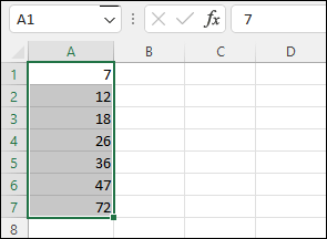
Start on a new blank spreadsheet. Now enter these arbitrary numbers in cells A1 to A7.
12 7 36 72 18 47 26
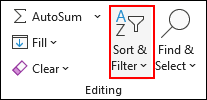
When you're doing quartiles, you need to sort your data, from lowest to highest. So highlight cells A1 to A7. In the Editing panel on the Home ribbon, select Sort & Filter > Sort Smallest to Largest:
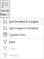
(You can also right-click the highlighted cells and select Sort > Sort Smallest to Largest from the menu that appears.)
Your spreadsheet should look like this:
OK, easy so far! Now to work out the formulas.
In statistics, the formula to get the first quartile is this:
(n + 1) / 4
The lowercase n is how many numbers are in your series. You add 1 to that and divide by 4. This will point to the number, but it won't tell you what that number is. For example, our number are these:
7 12 18 26 36 47 72
There are 7 numbers in all. So, n + 1 = 8. Divide that by 4 and you get 2. The 2 means the second number in your series, which is 12 in the series above.
Let's translate that to Excel.
In cell C1 of your spreadsheet, enter the text label First Quartile Row:. In cell D1, enter this formula:
= (COUNT(A1: A7) + 1) / 4
This counts how many cells are in the range A1 to A7, adds 1 to it, and then divides by 4. Press the enter key on your keyboard and you'll get a value of 2:
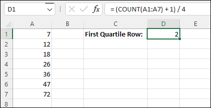
The 2 is the row number where the value is. So, the question is, How do you get a value in Excel using just a row number? Well, we can use the INDEX function for this.
First Quartile and The Index Function in Excel
If you want to get a value from a row number, INDEX comes in handy. You tell it what cells contains your values and then hand it a row number. Excel then returns the value you are pointing to.
So, in cell E1, enter the text First Quartile Value. Now enter the formula in cell F1:
=INDEX(A1:A7, D1)
When you press enter, you should see a value of 12 appear. This is the second number in our series. Here's what your spreadsheet should look like:
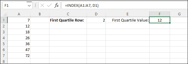
So, we've just found our first Quartile - 12. Let's do the second.
Second Quartile
The second quartile gives you the median value (middle one) of a series. The formula to calculate this in statistics is very similar to the one for the first quartile. It's this:
(n + 1) / 2
The only difference between the two is that we're now dividing by 2 instead of 4.
Back to Excel.
In cell C2, enter the text Second Quartile Row. Enter the following formula in cell D2:
=(COUNT(A1:A7) + 1) / 2
Press enter and you'll get a value of 4, meaning that the value is on row 4 of the spreadsheet. To get the actual value, we can use the same INDEX formula as before but with a different cell reference.
So, enter the text Second Quartile Value: in cell E2. In cell F2, enter this INDEX formula:
=INDEX(A1:A7, D2)
Press enter and your spreadsheet should look like this:
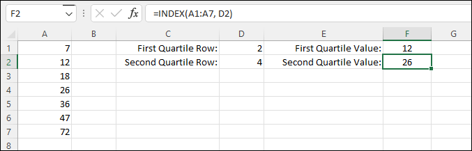
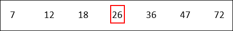
So 26 is the middle value (median) of our series of numbers, and it's on row 4 of column A. We have 3 numbers to the left of 26 and 3 numbers to the right of it:
Now let's get the third quartile and we're done.
Third Quartile
The third quartile gives you the other 25 percent of the entire quartile.
Q1: 25%
Q2: 50%
Q3: 25%
The formula for the 3rd quartile in statistics is this:
3(n + 1) / 4
This time, once you add 1 to n, you multiply by 3. Again, divide that answer by 4.
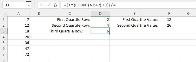
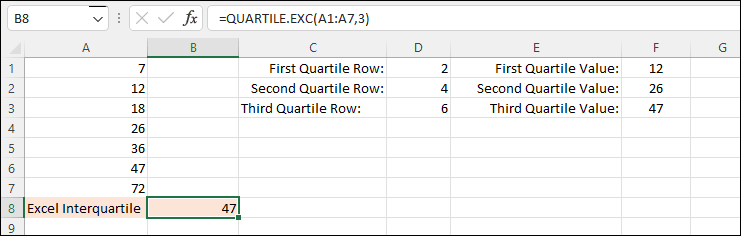
In Excel, enter the text Third Quartile Row: into cell C3. In cell D3, enter this formula:
= (3 * (COUNT(A1:A7) + 1)) / 4
Press enter to get the row number, which is 6 in our case. Here's your spreadsheet:
Again, we'll use cell D3 to get the actual value.
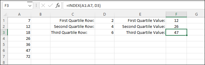
In cell E3, enter the Third Quartile Value:. In cell F3, enter this:
=INDEX(A1:A7, D3)
Press enter and you'll get the value from the A column, 47:
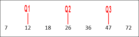
We now have three values for our three quartiles:
Q1: 12
Q2: 26
Q3: 47
If we spread our numbers out horizontally, you can get a better idea what it is we're doing:
After all that work, let's see how Excel handles it.
Click in cell A8. Enter the text Excel Interquartile:. In cell B8, enter the following formula:
=QUARTILE.EXC(A1:A7,3)
Press enter and you should get a value of 47:
QUARTILE.EXC stands for Quartile Exclusive. In between the round brackets of the function, you need the range of cells in your series. After a comma, type either 1, 2 or 3. The 3 we used is for the 3rd quartile. If you wanted the first quartile, enter 1 here. Enter 2 for the second quartile.
Excel has two quartile functions, one with EXC on the end, as used above,
and one with INC on the end. INC is short for Inclusive. The difference
between the two is that, for an odd number of digits in the series, EXC
excludes the median in both halves when calculating Q1 and Q3:
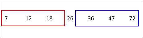
To get Q1, take the median of the first half above (the red rectangle). You get a Q1 value of 12 in the image above. To get Q3, take the median of the second half above (the blue rectangle). This gives you a Q3 value of 47.
For the INC function for an odd series of numbers, it includes the median in both halves:
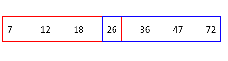
The Q1 value now is 15. It's 15 because you take the middle two numbers (median) of the red area, add them up, then divide by 2. So,
12 + 18 = 30
30 / 2 = 15
For Q3, the blue area, the value is 41.5. Add up 36 + 47, then divide by 2:
36 + 47 = 83
83 / 2 = 41.5
If there's an even number of values in your series, you just split them in half.
Interquartile Range
To calculate the interquartile range, you subtract Q1 from Q3. This will give two values, depending on whether you included the median or excluded it.
But type IQR in cell A10. In cell B10, enter this:
= F3 - F1
This gives you an interquartile range of 35. If you used INC with your formulas, you'd get an interquartile range of 26.5. So which excel function is best to use, EXC or INC? Well, it turns out that you can use either. In most cases, you get a very similar result. In some cases, you'll even get the same result. The results in this lesson were only different because we used an entirely arbitrary series of numbers.
In the next lesson below, you'll learn about standard deviation, which is a big topic in statistics. You'll then learn how the famous bell curve is created using Excel.
<--Back to the Excel Contents Page