Home and Learn: Microsoft Excel Course
Add an error message to an Excel Spreadsheet
In the previous part, you saw how to add drop down lists to your Excel spreadsheets. In this part, we'll display an error message for our users. If you haven't already done so, you need to do the previous tutorial first.
Data Validation - restricting what data can go in a cell
You can also restrict what goes in to a cell on your spreadsheet, and display an error message for your users. We'll do this with our Comments column. If users enter too much text, we'll let them know by displaying a suitable error box. Try the following:
- Highlight the E column on your spreadsheet (the Comments column)
- From the Data Tools panel, click Data Validation to bring up the dialogue box again
- From the Allow list, select Text length:

When you select Text Length from the list, you'll see three new areas appear:

What we're trying to do is to restrict the amount of text a user can input into any one cell on the Comments column. We'll restrict the text to between 0 and 25 characters.
The first of the new areas (Data) is exactly what we want - Between. For the minimum textbox, just type a 0 (zero) in there. For the maximum box, type 25. Your dialogue box should then look like this:

To add an error message, click the Error Alert tab at the top of the Data Validation dialogue box:
Make sure there is a tick in the box for "Show error alert after invalid data is entered".
You have three different Styles to choose from for your error message. Click the drop down list to see them:
In the Title textbox, type some text for the title of your error message.

Now click inside the error message field and type some text for the main body of your error message. This will tell the user what he or she did wrong:

Click OK on the Data Validation dialogue box when you're done.
To test out your new error message, click inside any cell in your Comments Column. Type a message longer than 25 characters. Press the enter key on your keyboard and you should see your error message appear:
As you can see, the user is prompted to Retry or Cancel. But our title (Too many characters) is at the top, our Stop symbol is to the left, and our Error message is displaying nicely!
Hiding Columns in Excel
The data that went in to our lists doesn't need to be on show for all to see. You can hide this text quite easily.
- Highlight the columns with your data in it (F, G and H for us)
- Click on the Home tab from the top of Excel
- Locate the Cells panel
- On the Cells panel, click on Format. You'll see the following menu:
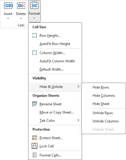
Click on Hide Columns from the Sub menu. Excel will hide the columns you selected:

In the spreadsheet above, the columns F to H are no longer visible.
To get them back again, highlight the columns E and I. From the same sub menu, click Unhide Columns.
In the next part below, you'll learn about something called circular reference.
<--Back to the Excel Contents Page