Home and Learn: Microsoft Excel Course
Business Invoice with Excel VLOOKUP, Part Two
In the previous lesson, you set up an Excel spreadsheet with three worksheets: Customer Data, Sales Data and Invoice. You have filled out the customer and sales data. It's now time to to set up the invoice.
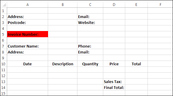
Click on your Invoice worksheet to select it. Create the following labels:

The cell A11, under Date, should be formatted as a date. Description and Quantity can be left on General. Price and Total should be formatted as Currency.
This is a very basic invoice, without any formatting. You can format it later, though, if you like. To start pulling data from the other two worksheets, we'll start with the Date, in cell A11.
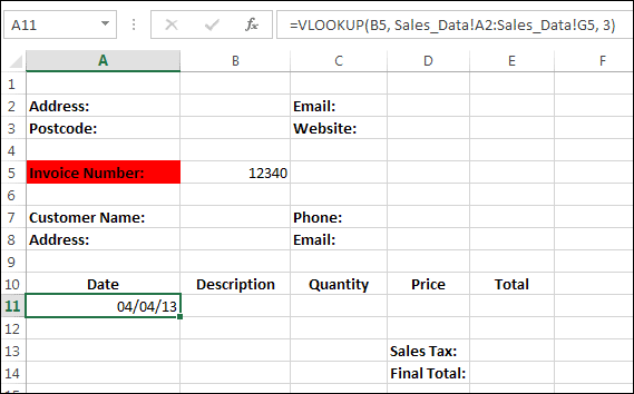
So click inside cell A11. Now enter the following VLOOKUP formula:
=VLOOKUP(B5, Sales_Data!A2:Sales_Data!G5, 3)
Just to refresh your memory, inside of the round brackets of the VLOOKUP function, we have three pieces of information:
VLOOKUP(value_to_lookup, data_to_search, results_column)
For us, the value we want to lookup is the invoice number in cell B5. The data to search can be found on the Sales_Data worksheet, in cells A2 to G5. (If you added more rows to your sales data then you need to change the G5 to whatever cell is the end of your data.) The column we want, the Date column, is column 3 (Column C).
After you've entered the formula, press the enter key on your keyboard. You should see #N/A appear. The N/A stands for Not Available. The result is not available because you haven't entered an invoice number yet. Do that now. Look at your Sales_Data worksheet and locate one of your invoice numbers. Return to the Invoice worksheet and enter your invoice number. Press the enter key on your keyboard and you should see a date appear in cell A11:

The VLOOKUP for the other headings (Description, Quantity, Price, and Total) are very similar. The only thing you need to do here is to change the column number for the final position. So the VLOOKUP function cell B11 would be this:
=VLOOKUP(B5, Sales_Data!A2:Sales_Data!G5, 4)
And the VLOOKUP function cell C11 would be this:
=VLOOKUP(B5, Sales_Data!A2:Sales_Data!G5, 5)
Cell D11 is this:
=VLOOKUP(B5, Sales_Data!A2:Sales_Data!G5, 6)
And cell E11 is this:
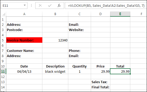
=VLOOKUP(B5, Sales_Data!A2:Sales_Data!G5, 7)
Enter the VLOOKUP function for yourself in these cells. Your spreadsheet should now look like this:

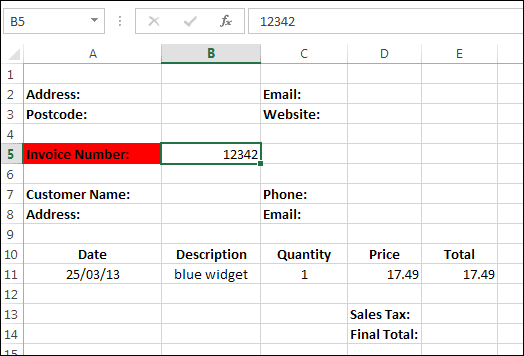
Now change your invoice number in cell B5. When you press the enter key on your keyboard, you should find that your invoice will update all by itself:

We now need to get the customer details for the invoice. This is more complicated. It's more complicated because we need to match a customer number from the Sales_Data worksheet to a customer number from the Customer_Data worksheet. We'll see how to do it in the final part, below.
Business Invoice Part Three -->
<--Back to the Excel Contents Page