Home and Learn: Microsoft Excel Course
Microsoft Excel Rows and Columns
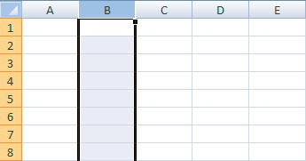
Spreadsheets are displayed in a grid layout. The letters across the top are Column headings. To highlight an entire Column, click on any of the letters. The image below shows the B Column highlighted:
If you look down the left side of the grid, you'll see numbers, which start at number 1 at the very top and go down to over a million. (The exact number of rows and columns are 1,048,576 rows and 16,384 columns. You've never going to need this many!) You can click a number to highlight an entire Row. If you look at the image below, you'll see that Row 5 has been highlighted
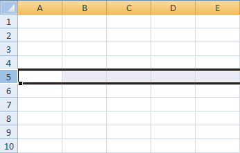
The image above is from a quite old version of Excel. Later are version are the same except less colourful. The one below is the one you'll probably see:

Spreadsheets are all about individual Cells. A Cell is a letter combined with a number. So if you combine the B column with Row 5, you get Cell B5. Combine Column D with Row 5 and you get Cell D5.
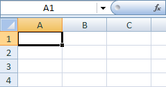

The first picture is Column A, Row 1 (A1), and the second picture is Column C Row 3 (C3). Notice that the cells we clicked on have a black border around them. This tells you the cell is active. The cell that is active will have its Column letter and Row number displayed in the top left, just above the letters A and B in the pictures. When you click into a cell, you can then type text and numbers.
To move around the spreadsheet, and make other cells active, you can either just click inside a Cell, or press the arrow keys on your keyboard. Try it now. Click inside a Cell and notice the Cell reference appear above the letters A and B. Press your arrow keys and notice how the active cells moves.
Before going any further, make sure you understand how the spreadsheet grid works. If you are asked to locate Cell H2, you should be able to do so.
We'll now enter some simple data into an active cell.
Entering Text and Numbers in a Cell -->
<--Back to the Excel Contents Page