Home and Learn: Data Analysis
Basic Pandas Operations
In the previous lesson, you imported a CSV file and loaded it into a Pandas DataFrame. In this lesson, you'll learn basic operations you can perform on your Pandas data. Let's start with Shape an Info. If you haven't done this lesson, here's a CSV file for you to download. (CSV stands for comma separated values.)
Download the Pets Data CSV File (Right-click, Save As)
Once you've downloaded the file, copy and paste the following code into a new cell in a Jupyter Notebook:
import pandas as pd
df_pet = pd.read_csv('PATH_TO_FILE.csv')
df_pets
Replace PATH_TO_FILE with wherever you saved your downloaded file to.
Pandas Shape
Whenever you first read a csv file in and create a Dataframe, you'll want to display basic information about the Dataframe. We'll go through some of the methods you can use.
If you want to display how many rows and columns you have in the Dataframe, you can use shape. Enter the following into an empty cell in your notebook (this assumes you are following along from the previous lesson and have created the df_pets DataFrame.):
df_pets.shape
Shape is an attribute of Dataframes, rather than a method or function, so it doesn't need round brackets.
Press Run at the top of your Jupyter Notebook and you should see this:
df_pets.shape
(27, 4)
The first number between the round brackets is how many rows you have in your Dataframe. The second number is how many columns you have.
Pandas Info
To get information about the Dataframe, you can use the function info(). Enter the following into an empty cell in your Notebook:
df_pets.info()
You should see this when you click the Run button (or press CTRL + ENTER
on your keyboard as a shortcut.):

OK, so what is it telling us here?
Well, we learn that the Range Index goes from 0 to 26, which is a total of 27 entries. The total number of columns is 4. Then we get a table printed out. The table tells us what the name of the columns are: Pet, OwnerGender, OwnerAge, and PetAge. We also learn that there are something called non-null values, and Dtypes (we'll get to these Dtypes an null values in a later lesson).
Let's see how you can rename a column.
Rename Columns in Pandas
Let's rename the Pet column. To get a list of all your column names, you can use the columns attribute (no round brackets on the end as it's not a function or method). Add this line to an empty cell in your Notebook:
df_pets.columns
You should this, when you run the code:
Index(['Pet', 'OwnerGender', 'OwnerAge', 'PetAge'], dtype='object')
To rename columns, you use the rename function (note the round brackets on the end):
df_pets.rename()
Except, you need something in between the round brackets of rename. You need the word columns, followed by an equal sign. After the equal sign, you need a Python dictionary. If you're not familiar with Python dictionaries, they look like this:
{'KeyName': 'KeyValue'}
It's just a pair of curly brackeys with a key name and a value for the key.
In Pandas, you type the name of the column you want to rename, surrounding by quote marks. After a colon, you need a new name for the column, again, surrounded by quote marks. Here's some code to enter into a new cell in your Notebook:
df_pets.rename(columns={'Pet': 'PetType'}, inplace=True)
df_pets.columns
The inplace=True at the end (you need a comma after the final curly bracket) means that the original file will be amended. If you didn't add this, you'd just get a copy and the underlying Dataframe would remain unchanged.
When you run the code, you should see this:
Index(['PetType', 'OwnerGender', 'OwnerAge', 'PetAge'], dtype='object')
You can rename more than one column at a time. Just added more items to your dictionary:
df_pets.rename(columns={'Pet': 'PetType', 'OwnerGender': 'GenderOfPetOwner'}, inplace=True)
Display the first five rows of your Dataframe, though:
df_pets.head()
You should now have this:

Remove Duplicate Rows in Pandas
You'll want to know if your Dataframe contains duplicate rows. To check, use the duplicated function:
df_pets.duplicated()
If you were to run this line in a new Notebook cell, you'd see that you get back a series of True or False values. To get the actual results for all rows, you would need to run this line:
df_pets[df_pets.duplicated()]
You need the name of your Dataframe first, then a pair of square brackets. Inside the square brackets, you need the dataframe name again followed by the duplicated function. When you run the command, you'd see a table listing any duplicated values. There are no duplicates in our data set, so the table will be empty, and you'll just see the column names.
You can get rid of duplicate rows quite easily by using the function drop_duplicates.
df_pets.drop_duplicates(inplace=True)
To see the results, you'd typically run the shape aommand again:
df_pets.shape
When the shape command runs, you should find that you have fewer rows than when you started.
Basic Aggregate Function in Pandas
Aggregate functions are ones like sum, mean, count, max, min. Let's see how they work.
Suppose you wanted to know the mean age of all the pet owners. You could do it like this:
df_pets['OwnerAge'].mean()
You need your Dataframe name (df_pets), then a pair of square brackets:
df_pets[ ]
Inside the square brackets, type a column name surround with quote marks:
df_pets['OwnerAge']
The aggregate function you want to use goes after the square brackets. Type a dot, then the name of the aggragate function you want to use, not forgetting the empty round brackets on the end:
df_pets['OwnerAge'].mean()
Run that line in a new empty cell in your Jupyter Notebook. You should see this:
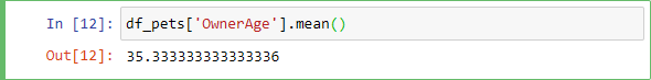
So the mean age of the pet owners in our data set is just over 35.
Now try some of these:
df_pets['PetAge'].mean()
df_pets['OwnerAge'].count()
df_pets['OwnerAge'].sum()
df_pets['OwnerAge'].max()
df_pets['OwnerAge'].min()
(The count function tells you how many rows are being counted.)
Here is a fuller list of the aggregate functions, should you need them:
| Aggregate Name | Explanation |
| count | counts the values in a column. Ignores null values. |
| min | minimum value in the column |
| max | maximum value in the column |
| first | first value for a category |
| last | last value for a category |
| std | standard deviation |
| sum | sum of values in a column |
| mean | the mean of the column values |
| median | the median of the column values |
| mode | the mode of the column values |
| var | variance (unbiased ) |
| mad | the mean of the absolute deviation |
| quantile | the quantile of the column values |
| skew | skew ( unbiased) |
| sem | standard error of the mean |
| unique | unique values in a group |
| nunique | Get a count number of the unique values in a column |
One all rounder for looking at aggregate statistics is the describe function. Try this in a new cell:
df_pets['OwnerAge'].describe()
When you run the command, you should see a table of basics stats, like count, mean, min. max, etc.
Running more than one Pandas Aggregate Functions at a time
You can run more than one aggregate function at a time, if you want. This time, however, you need to use the agg function after the name of your Dataframe:
df_pets.agg()
In between the round brackets, you need one of those python dictionaries again:
df_pets.agg( { } )
To get the mean, min, and max of the pet owner, add the column name in quote marks then a a colon:
df_pets.agg( { 'OwnerAge' : } )
After the colon, you can add your aggregate functions in square brackets:
df_pets.agg( { 'OwnerAge' : ['mean', 'min', 'max'] } )
Run the above code and you should see a table appear:

You can add more than one column. Just add a comma after the square bracket, then the new column and functions. Try this:
df_pets.agg( { 'OwnerAge' : ['mean', 'min', 'max'], 'PetAge': ['mean', 'min', 'max'] } )
Run the command to see the new table:

Pandas value_counts()
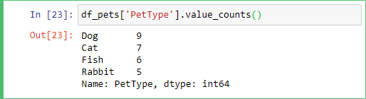
One very useful function you can use is called value_counts. As its name suggests, you use to count values in your data set. As an example, try this in a new cell in your Jupyter Notebook:
df_pets['PetType'].value_counts()
You should see this as the result:
So, you need the name of your Dataframe and a column name between square brackets:
df_pets['PetType']
After a dot, type the function name and its round brackets:
df_pets['PetType'].value_counts()
You get a count of all the values in the series that don't have null values (see next lesson for a deeper dive into null values). The display is in descending order. So, the count of 9 comes first here. It's counting how many times the PetType Dog was recorded.
If you want the display in ascending order, you need to add ascending=True between the round brackets of value_counts. Try this;
df_pets['PetType'].value_counts(ascending=True)
The result is this:

This time, 5 is the value at the top and the PetType is Rabbit.
You can do an alphabetical sort of the values. You just need to add a new function on the end - sort_index. Try this:
df_pets['PetType'].value_counts().sort_index(ascending=True)
The results is this:

Now the PetTypes are sorted alphabetically. Cat comes first because we specified that ascending=True. If you miss this out, you get a descending sort and Rabbit would be top.
If you want an alphabetical sort when some of the values are equal, you need to add yet another function on the end:
df_pets['PetType'].value_counts().sort_index().sort_values()
The new function is sort_values. If we had, say Fish and Rabbit at both 6 for their count, then the PetTypes aould be sorted alphabetically in the results.
You can also display the values as percentages. Try this:
df_pets['PetType'].value_counts(normalize=True)
By using normalize=True between the round brackets of value_counts, you get a percentage figure:

Now that you've gotten the hang of the basics, let's move on. We'll take a look at null values, because you'll get a lot of them in your own data sets, and you need to know how to deal with them.